Logistic & Probit Regression: Predicting a Binary Outcome Variable

Note: this post is part of a series of posts about Categorical Data Analysis: Dealing with Counts, Frequencies & Percentages

Previously, we have been looking at count data (yes/no). At times, we even aggregate count data into a proportion (%). But fundamentally — these still are group comparisons. Instead of analysing how a dependent variable changes across groups, is there a way to analyse how a dependent variable changes across a continuous variable?

Logistic Regression: Continuous IV, Binary DV

For those unfamiliar with the terminology — IV stands for Independent Variable, while DV stands for Dependent Variable. Typically, when we analyse for relationships between variables, we think of it as predictor variables (IV) predicting outcome variables (DV). Which means there’s a direction to your relationship — in that it is the IV that is affecting your DV.

In the Chi-Square Test of Analysis and the Two Sample Test for Proportions — this “directional relationship” isn’t as obvious. As we all know — correlation is not causation — and it’s often difficult to conduct true experimental studies to prove causation when it comes to categorical variables (e.g. gender, job type, SES etc).

But when it comes to continuous variables — the notion that one factor precedes the other becomes obvious. Whether it is time spent job hunting on job success, years in the workforce and being in senior management — flipping the IV/DV just no longer makes as much sense. Thus, for Logistic Regression, it becomes important that you are clear in your head what you are trying to prove — that it is the IV affecting the DV, and not the other way around.

Logistic Regression as a Linear Model

In R — you can easily call the Logistic Regression function via

model = glm(y ~ x, data = df, family = "binomial")

Notice what R calls it — GLM. GLM stands for generalised linear model — implying that at its core, logistic regression is still a LINEAR MODEL. (I’ve actually already wrote about this in another post over here — do check it out!)

The idea is that we want to keep the normal linear regression framework to predict a response variable that only takes values between 1 and 0. Thus, by transforming the variable slightly, we get this equation:

This is in linear regression format (notice the right hand side is completely like a normal linear regression). Shifting the terms around slightly, we then get this equation — corresponding to this graph:

Notice that the y-axis range now nicely fits even 0 and 1 — which is exactly how we want the variable to behave!

Is Logistic Regression the Only Appropriate Function for Binary Outcomes?

No! If you really think about it — all you need to do to use regression to predict binary outcomes is to “scale” the predictions somehow into the range of 0 and 1. While Logistic Functions do so via transforming the predictor variable via odds and log transform, another possible way to do so is via a normal distribution.

Probit Regression: Alternative to Logistic Regression, Based on Normal Distribution

Follow my argument for a bit. Let’s assume that the classification is fundamentally determined by an unobserved (latent) normal variable. And as such, our regression equation actually predicts these unobserved z-values instead (this works because z values range from negative infinity to infinity as well).

Thereafter, converting the z-values to probabilities is child’s play. Since the total area under a z-curve is 1, we can compute the corresponding probability tagged to that particular z-value — and then use this probability as the probability of being Y = 1.

To give you an example — say my observed z-value was 1.25. The corresponding area under the curve would be 0.8944, and thus this is the predicted probability of being Y = 1.

The mapping of the z-value to the probability under the curve can be done via the normal cumulative density function (CDF) — which is just a fancy equation to find the area under the curve (I find that sometimes people are so intimidated by the name of the function that they fail to understand that it’s actually a very simple thing haha)

And so — the coefficients of your predictor variable in a Probit Regression Model actually represent the change in the latent z-score — which then can be converted into a corresponding probability being success. Obviously, the corresponding probability does NOT change linearity because the z-distribution is a curve — meaning the every unit increase in z-score does NOT lead to an identical increase in probability.

The normal CDF function is often written mysteriously as a phi symbol — contributing to why people think it’s very difficult. But honestly — we write it that way because the full equation is messy — not because we are trying to be mysterious.

Logistic Regression and Probit Regression: Fundamental Differences

Why have so many different methods for the same thing? Truth is, I can’t answer this question well. The question I instead would pose to you is — if you chose one method over the other, what’s the basis for that decision?

It’s precisely because there’s no strong justification about favoring 1 over the other — that there exists so many methods for the same thing. The “base” models for the Logistic and Probit Regression models look slightly different:

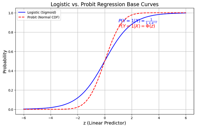
But naturally during the regression fitting you can adjust the steepness of these curves such that they may end up aligning rather strongly with each other.

There probably are simulation studies out there which outline the specific situations in which a Logistic is more appropriate than a Probit or vice-versa — but honestly for the most part, they do tend to give similar results.

The Nuances of Model Selection

Which again brings me to my point — there’s no one way to model a dataset!

As we first explore the world — impressed by all the messiness and wonders of it — we set out believing that it can never fully be understood and that science is just a way of understanding the world.

When you first learn about statistics — just by virtue of the fact that you only know a few models — you start to believe that these models are the be all and end all — and that models are the only window into the world.

Then only as you progress further in your journey, you learn more statistical tools — you realise that each model is like a kind of window into the world — offering unique insights and perspectives. They sometimes lead you to see very different things — but that does not mean that either of the models are wrong as well. And it is only at this point — you start to realise that choosing a statistical model is like choosing which window to look through — any window you pick actually has alternative, feasible windows that might be worth exploring as well.

Credits to: https://imgflip.com/memegenerator/312904212/Normal-Distribution-meme

The choice of model also affects the significance of your predictor — so if you are interested in a p-value interpretation — do be mindful of this! A predictor may be significant under the logit link but not significant under the probit link — this is just a fact you will have to acknowledge when fitting your model. (p-values aren’t that straightforward anymore, are they heh)

Conclusion

And with that — you now have 2 new tools you can use to analyse data! Probit and Logistic Regression are most useful when you have a continuous IV and a binary DV.

In the next post, we’ll look at simple extensions of the Logistic Model — because the DV we want to predict isn’t always going to nicely be binary — we sometimes have DVs of 3 or more categories.