Time Series Analysis Made Simple: From Regression to Markov Chains

Note: this post is part of a series of posts about Data Analysis In The Real World

If you have graduated and are analysing real world datasets — you would have realised one thing very quickly. Virtually all the datasets you receive now are timestamped — and your bosses are often interested to know how the trend is changing over time.

Analysing Time Series Data: What a Beginner Would Do

Of course — descriptive analysis is no kick at all. It’s easy to just sum/average things across days/months/years — then just chart things out over your desired period of time. A simple example would be say — how has my sales been like for the last 2 years?

Say you are, Nike for instance. The sample dataset can be found here.

You are interested in seeing how the sales of your shoes have been doing over the past two years. You plot out a chart at the monthly level for your boss. Say the chart looks like that.

The million dollar question then comes from your CEO: “have our shoe sales really been increasing? It seems like the increase isn’t that big.”

Everyone then turns to you — the data analyst/statistician/data scientist. Silence in the meeting room, as people wait for you to utter your words of wisdom.

Credits to imgflip.com

Hahaaha I guess I always had something for dramatic moments. But literary imagery aside — the bigger question still remains. How would you answer the CEO’s question?

Side note: Okay. Perhaps I should confess— the way I presented the CEO’s question was already in a very statistical format — because… well.. I want to talk about statistics! Truth is, the actual question I got was “what would the sales look like in 2026” — which is an entirely different question altogether. Let’s stick with my statistical question for now first.

Any thoughts on how to properly analyse if your sales have been increasing? If my guess is correct — the majority of readers would choose a simple linear regression model — whereby you regress your shoe sales against time — and then test to see if the slope is significantly different from 0 (of course, different in the positive direction).

Force Fitting Time as a Predictor in a Regression Model

But the question then becomes: How do you make time an independent variable? Can time even be an independent variable? What kind of scale would that be?

Clearly — it is not a typical continuous variable as is say, height. You know it is a “continuous” variable — but January, February, March isn’t exactly a measurement scale you learn it school (lol). What do you do then?

I’ll tell you what I did. Since we know our linear regression model typically works with numbers — we need to convert our date data into numbers as well. I created a new variable titled “months since Jan 2024” — then re-coded the date data into (0,1,2,3…. 23). And now, I can regress shoe sales against time in the format we are very used to.

Notice something important? Descriptively, your time variable already has a negative relationship with shoe sales (coef = -0.317). Plotting out the best fit line along with the original data, we get this:

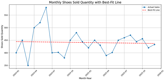
We can see that the CEO’s suspicions were right — truth is, our sales does not really seem to be increasing with time. Instead, the best fit line suggests that it is decreasing.

This decrease was not significant though — meaning that at best, we can claim that our sales have not changed (no evidence against the null hypothesis to be precise, but not bombarding your audience with overly technical details is important you know).

To put it out explicitly — what I did was that I basically created my own interval scale for the date data. Since an interval scale is a form of continuous measurement scale, we can then easily use our date data as a predictor of shoe sales via regression.

Is the Regression Model Valid?

But pause for a moment now. Does something feel off to you? Compare your IV to a more typical IV you would have used in school. Is drug dosage of 5ml, 10ml, 15ml really identical to Jan, Feb, Mar? Is the relationship between 5ml vs 10ml identical to the relationship between Jan vs Feb?

The point I’m trying to make here actually ties back to the most fundamental assumptions of the Linear Regression method: Independence of Datapoints. In a typical experimental setting — we randomly assign participants to the 5ml, 10ml, 15ml conditions. Each of these datapoints are assumed to be independent — and there is no real relationship between a datapoint in the 5ml condition to another datapoint in the 10ml condition.

Side note: Even if we cannot randomly assign participants — we can still do a quasi-experimental design. Things like gender (male vs female) — sure they cannot be randomly assigned, but the independence assumption still holds — you would not expect any form of relationship between a datapoint in the male group and a datapoint in the female group!

But can the same really be said for a datapoint in Jan, vs the datapint in Feb? Is the sales quantity of the next month really independent of the sales value of the previous month?

Violation of Independence Assumption — Auto-Correlation

In school, the only context we learnt in which the independnece assumption was violated is via paired data (repeated measures from same participant). Now, allow me to introduce you to another form of independence violation — autocorrelation.

Autocorrelation means that (the residual of) a datapoint is correlated with the lagged version of itself. What exactly does that mean? Notice that the data we are collecting is the SAME throughout the entire dataset — the quantity of shoes sold.

In Times Series Analysis, we view our dependent variable as not as multiple measurements from the same participant (as for paired data in research) — but multiple measurements of the literally the same thing. Which is why we term the quantity of shoes sold in Janurary as a lagged version of the quantity of shoes sold in Feburary.

Lagged Version of Itself — Mathematically

We often denote the measurement at the current time as x(t), and the measurement at the previous time x(t-1). So assuming you are in Feburary, the quantity of shoes sold in Feb would be x(t), and the quantity of shoes sold in Jan would he x(t-1). (Pardon the inability to subscript on medium!)

Everything is defined with respect to the current time frame. So if you are now in Mar — the quantity of shoes sold would now be x(t), and the quantity of shoes sold in Feb becomes x(t-1). And so on for Apr, May, June.

Autocorrelation simply means that a variable is correlated with lagged versions of itself. For instance, x(t) has may have a correlation with x(t-1).

This is still exactly the same correlation we learnt in school — just that instead of a correlation between 2 separate variables, we are now looking at the correlation between something and a lagged version ot itself.

AutoRegressive (Markov) Models

Now that we understand autocorrelation — we can go on to use this knowledge to create autoregressive models. Becuase think about it — what does autocorrelation mean? It basically means that there is a relationship between the current measurement and lagged versions of itself. In other words, we can use the previous measurements to predict (to some extent) the current measurement via regression.

Side note: This jump from autocorrelation to autoregression is exactly the same as the transition from correlation to regression you learnt back in school!

Of course — there are possibly an infinite number of “previous measurements” — it really just depends on how much data you have. Most commonly, we assume that the current measurement (xt) is only predicted by the most recent previous measurment (xt-1). This gives us the most common (and famous) time seires model, known as the (1st order) Markov Model — which looks something like that:

Fancy as the name sounds, the meaning is simple really. The first thing you need to notice is that it looks suspiciously similar to your typical regression model. And indeed, that’s because he interpretation is exactly the same!

Markov Model simple states that the current mesaurenet can be predicted solely by the previous measurement (not related to previous states further than this). To run this model — of course there are softwares/codes to do so. However, I feel that the best way for you to truly understand what you are doing would be to manually create your dataset and use your typical regression module to test the model. So follow along with me as I run you through this process.

Our dataset actually looks like that:

This data structure follows the tpyiclaly IV/DV interpretation we are used to — because we view time (month) as our IV, and quantity of shoes sold as our DV.

However — we need to remember that the theoretical rationale for this data format is actually when the IV and DV are completely different construscts. Typically, the IV is like “Study Time”, and the DV is “grades”.

But in this setting — technically, the IV is already implicit within the “order” of the DV. Even without the “IV” column — we can infer the the month based on which position the measurement is in.

Which is why — we could present our data like that — in a single column alone — wihtout any true data loss.

But with 1 column — how do you run a regression analysis? You can’t. Which is why, to crate your x(t-1) predictor — create a new column, copy and paste all the x values, and shift it down by 1.

Boom! Mind blown! It’s so simple — yet it feels like we are in a completely new realm of regression right now. You should notice that your IV now always contains the measurement from the preceding month (IV is Jan when DV is Feb, IV is Feb when DV is Mar). Of course — we can ignore the top most and bottom most measurements since there are blanks in these — and regression can’t accept blank values.

And now — just simpy run your normal regerssoin with x(t-1) as your IV, and x(t) as your DV!

PS: did I just use excel to run regression?!? Yes. Yes I did.

Congratulations! You just fitted a time series analysis model!

Durbin Watson Test for Autocorrelation

In the first regression model we fitted (with month as the predictor and shoes sold as the DV) — you might have noticed that in your regression output there’s this Statstic called Durbin Watson.

Truth is, the Markov model you just fit actually is what the Durbin Watson statistic “represents”. The Durbin Watson Statistic is a test for (1st order) autocorrelation— wth a value of 2 indicating no autocorrelation. Values closer to 0 suggest positive autocorrelation, whereas values closer to 4 incidate negative autocorrelation.

When the value deviates too far from 2 — that suggests that autocorelation is present, and that your indepedence assumption does not hold. In the above dataset, the value of 1.6 is still rather close to 2 (heuristic judgement) — which means that even though theoretically the datapoints are related, empirically the independence assumption seems to hold.

And as such — this means that in this case, your initially regression model would actually have worked out just fine (supported by that fact that your Markov Model did not reach significance as well).

Final Note about Time Series Analysis

Everything I’ve said above is all good and dandy. However, once you enter into the realm of time series analysis, the goal of your analysis likely starts to change (as alluded to earlier).

More typically, your goal shifts from proving a relationship (statistics) to predicting future values (machine learning). Because think about it — “time” isn’t really a strong “explanatory” variable, is it? It’s not like dosage of drug — where there actually is a purpose in proving that the IV affects the DV. For IVs like time — it’s more like a… oh. Okay sure — so what?

Instead, when time is your IV, people are often more interested in forecasting future values — whether it is sales, demand, or even stock prices. Which is why in Time Series Analysis, true blue statistical techniques like SARIMA/SARMIAX are less often used then fancy machine learning models like RNN or LSTM. Because at this point — you don’t really care about relationships between variables — you just want to know the prediction.

Want to learn about these more advanced techniques? Subscribe to my Telegram Channel and Medium Posts! Hahaha.

Stay tuned — my dear readers!