Geospatial Analysis: The Basics

What is geospatial analysis? You should already have gotten a taste of it from my Primer Article here. Simply put, it is about finding insights based on location data.

For the vast majority of students - geospatial analysis is not something you learn in university because it is rather specialised. However, you will likely deal with it in the course of being a data professional - because your customers come from geographical regions, your stores have a location, everything occurs somewhere. Point is (pun intended) - you can’t escape from geographical data!

So let’s go ahead and get our fundamentals in first. Let’s talk about the common data types, how data is typically processed, and what these data actually mean.

Geospatial Data Types: Vector vs Raster Data

The very first distinction we need to make is about Vector vs Raster Data. It’s different to verbally explain the difference between these 2 data types - because they are just categorically different from each other. It is much easier to just illustrate, so here is a picture:

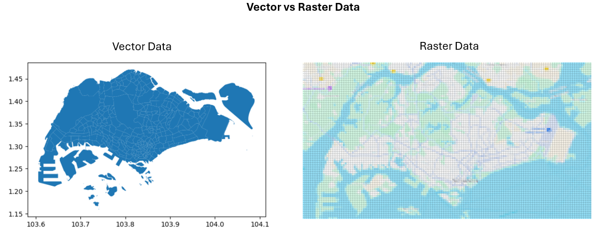
Vector Data is mathematical. It is literally points, lines & shapes. They can be zoomed in on without any loss in quality. The data files come in the form of SHP files, GEOJSON etc.

Raster Data is literally “pictures”, if you will. Typically some call them raster “tiles” - whereby each tile is made up of pixels. So raster data is literally made up of tiny squares - each of which has a value (whether brightness, intensity, RGB or whatsoever). Which naturally means that if you zoom in, there WILL be loss of quality. These usually come in GeoTIFF file extensions.

When you do geographical analysis - you will usually overlay multiple layers on top of each other. The most common forms would be layering vector on vector, or vector on raster. This is because you will typically have a vector layer of points (your data of interest), and you want to visualise it on a base map (can be vector or raster). This is what helps give you location based insights to your analysis.

Coordinate Reference Systems: Projected vs Geographic CRS

Points are an excellent example of vector data. They are mathematical, and oftentimes we see numbers attached to them. But what do these numbers represent? To understand these, we first have to be clear about Coordinate Reference Systems (CRS).

There are technical definitions of these, but let’s just get the intuition in. Think of how you would define a place in a spherical earth. Obviously, this is hard because the earth is 3D. One thing that helps, however, is that land areas are all on the surface of the sphere - so you don’t need an additional z-axis. x and y will do.

In order to define the X and Y planes, the first thing you need to do is define where your “center” is. Intuitively, you would define it with respect to the largest plane within each axis - right smack at the center. Indeed - this is exactly the equator (central horizontal line) and the central meridian (the central vertical line).

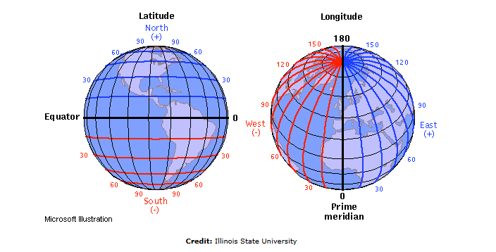
Taken from https://archive.journeynorth.org/tm/LongitudeIntro.html, from Illinois State University

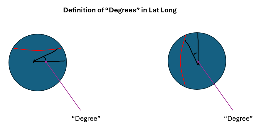
Since the earth is a sphere - these lines have to be defined with respect to DEGREES from the center (centroid of sphere) - if you imagine drawing a triangle for every ring position and the angle of that triangle being the defining degree of that line (see below).

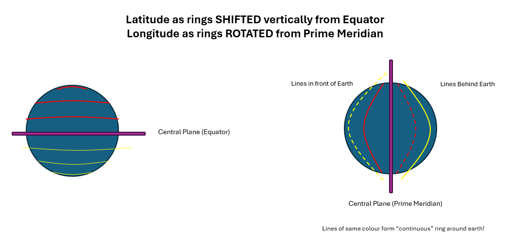
The funny thing about these vertical & horizontal lines, however, is that they are not defined equally. While they are both measured in degrees from the center, only longitudes (the vertical lines) are actually rings rotated from the central plane. Instead, latitudes (horizontal lines) are literally rings shifted up and down of the central plane (the rings thus get smaller & smaller the further they go from the equator, before converging into a point at the tip of the earth.

And yet still - even with this system, the intersection between the lat long is still not a point. Instead, it is 2 points, because if you image any latitude ring running horizontally - another vertical longitude ring will intersect the horizontal ring exactly twice.

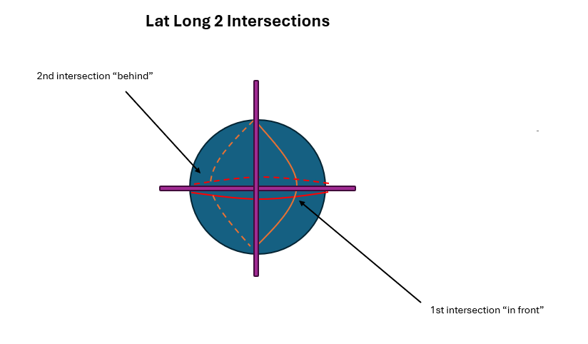
Which is why - longitude rings are not exactly complete “rings”. Instead, each half of the ring has a different sign (positive and negative) - which helps make the system define the intersection as 1 point exactly.

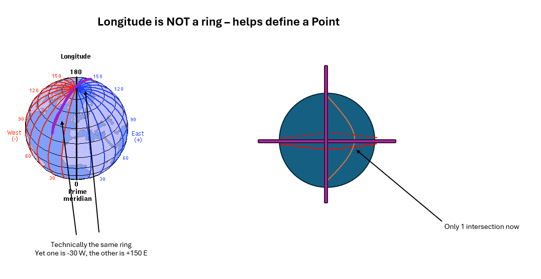
Great! We now know how lat long works!

Side note: even though “lat long” got popularized as a term, this is actually “y x” - which goes against cartesian convention. More specialized GIS software actually requires you to input the data at long lat (x, y)! It gets confusing because the vertical lines are defined with respect to x degrees (horizontal rotation axis), while the horizontal lines are defined with respect to y degrees (vertical rotation axis).

Lat Long is an example of a Geographical Reference System - which deals directly with the fact that the earth is 3D. But unless the distances are really very huge, within each locality, oftentimes we can approximate the map to be 2D (stretch it out) without much implication. And indeed this makes life a lot easier - because the units can directly be in terms of meters, instead of degrees.

The 2D flat map approach is known as the projected reference system. Intuitively, we all already know how it works. Just define a nearby point as 0 - then define any place with respect to how far this point is away from the reference point (in terms of x and y distance, now directly in meters).

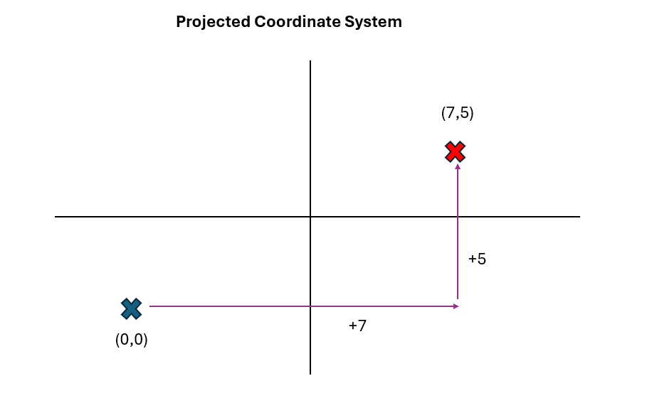
Depending on which region you are in, you typically choose a Projected reference system that is suitable for your locality - to ensure that the 2D distance remains a good approximation of the distances!

When we work with any GIS software - we will always have to specify which CRS we are using. EPSG:4326 stands for the lat long convention - which is typically how most analyses start. From here, we convert the data into the Projected CRS of interest, then go about our distance computations (if necessary). 

Conclusion:

Great! You’ve gotten the solid fundamentals of geospatial analysis - and now know what the data types are and what they usually mean. Don’t get too happy though - we still have a lot to do! Let’s dive right in and proceed to overlay some points (vector data) on a map (can be vector or raster) - and get a taste of our very first location-based insight from a dataset.

Stay tuned! 😀

Note: This post is part of a series of posts regarding Geospatial Data Analysis